I have been recently working on a paper about the short-term car registration forecasting. Forecasting models were based on several underlying variables which were analysed by a standard Vector Autoregressive Model. As the main purpose of the paper was not to present a black-box model with a good predictive power, we needed to analyse leading indicators. A traditional approach to identify “cause and effects” in the context of time series analysis is to perform the Granger Causality test. Causality in this context means that an inclusion of the variable reduces a MSE error. Some variables might be only good signals - not a true underlying causes of car registrations.
Surprisingly, a treatment of the multivariate Granger-causality concept is not discussed much. Typically, two variables settings is presented with the caveat that solution works even for a more variables. This is only a partially true.
In the following text we will go through the simple 3 time-series example with various settings of interconnections. Let’s start with stationary time-series only.
Three Variables, One driver
This example shows the analysis of the tree time series where the first time series ts1 is a confounding time series.
The first time series (TS1) is generated as an autoregressive proces AR(1):
library(dplyr) # for %>%

ts1 <-  stats::arima.sim(n = 100, list(ar = c(0.7)), sd = 1/2) %>% as.numeric
The second time series TS2 is computed as a standalone AR(1) process plus TS2 multiplied by value . Similarly, TS3 is based only on its own autoregressive part plus values.
alpha <- 0.7
beta  <- 0.7

set.seed(123)
ts2 <- arima.sim(n = 100, list(ar = c(0.7)), sd = 1/2) + alpha * dplyr::lag(ts1, 1)
ts3 <- arima.sim(n = 100, list(ar = c(0.7)), sd = 1/2) + beta * dplyr::lag(ts1, 1)

ts1 <- ts1 %>% as.numeric
ts2 <- ts2 %>% as.numeric
This settings can be visualised in the diagram:
library(DiagrammeR)

DiagrammeR::grViz("
 digraph boxes_and_circles {

 graph [overlap = false, fontsize = 1, rankdir='LR']

 TS1 -> TS2 [label = 'AR1 + α·TS1']
 TS2 -> TS3 [label = 'No Relation', color= 'red', fontcolor='red']
 TS1 -> TS3 [label = 'AR1 + β·TS1']
}
")What should we expect to see now? TS1 causes TS3 as it is a function of TS plus an indepedent AR(1) process. TS1 causes TS2 for the very same reason. Therefore, there should be a strong correlation between TS2 and TS3. Again, TS2 is just a variable which consists of information from TS1 plus indepedent AR(1). The sole “effect” of TS2 is just an AR(1) process which is masked by the influence of TS1.
This data-generating process is unkown to the analyst. Let’s assume the analyst is not aware of the TS1 and observes only TS2 and TS3.
library(ggplot2)
library(tidyr)

data.frame(ts2, ts3) %>%
  dplyr::mutate(Date = seq(as.Date("2000/1/1"), by = "month", length.out = 100))%>%
  tidyr::gather(TS, Value, -Date) %>%
   ggplot(., aes(x=Date, y=Value, colour=TS) ) +
    geom_point() + geom_line() + theme_bw()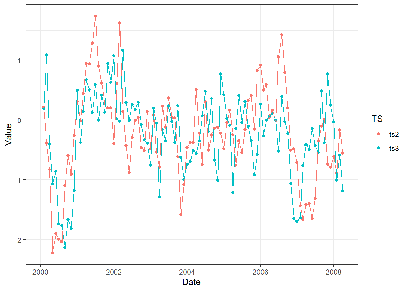
We will skip formal testing of stationarity. Let’s fit the Vector Autoregressive Model.
library(vars)
library(broom)
varData1 <- data.frame(ts2, ts3)
varFit1  <- vars::VAR(y=varData1[-1, ])
We are interested in the part of the VAR where the TS3 is a dependent variable.
library(knitr)
library(kableExtra)

tidy(varFit1$varresult$ts3) %>%
  knitr::kable(digits=3) %>%
kableExtra::kable_styling(bootstrap_options = "striped", full_width = F)| term | estimate | std.error | statistic | p.value |
|---|---|---|---|---|
| ts2.l1 | 0.269 | 0.081 | 3.303 | 0.001 |
| ts3.l1 | 0.438 | 0.092 | 4.783 | 0.000 |
| const | -0.090 | 0.059 | -1.535 | 0.128 |
Both the lagged variable of TS3 and TS2 were indetified as statistically significant. Let’s approach to the actual Granger Causality test. There is a function called vars::causality which performs F-type Granger test. Our model was identified as VAR(1) since the only variables of lag 1 were chosen as optimal (according the to AIC criteria).
This function is quite straigtforward:
causality(varFit1, cause = "ts2")$Granger # there is also Instantaneous test in .$Instant##
## Granger causality H0: ts2 do not Granger-cause ts3
##
## data: VAR object varFit1
## F-Test = 10.91, df1 = 1, df2 = 190, p-value = 0.001143We can reject the null and can claim there is an evidence for TS2 Granger-Causes TS3. This is exactly what we have expected.
grViz("
 digraph boxes_and_circles {

 graph [overlap = false, fontsize = 1, rankdir='LR']

 TS1 -> TS2 [label = 'AR1 + α·TS1']
 TS2 -> TS3 [label = 'AR1 + γ·TS2']
 TS1 -> TS3 [label = 'AR1 + β·TS1']
}
")gamma <- 0.7
ts1 <- arima.sim(n = 100, list(ar = c(0.7)), sd = 1/2) %>% as.numeric
ts2 <- arima.sim(n = 100, list(ar = c(0.7)), sd = 1/2) +
alpha * dplyr::lag(ts1, 1) %>% as.numeric
ts3 <- arima.sim(n = 100, list(ar = c(0.7)), sd = 1/2) +
beta * dplyr::lag(ts1, 1) + c(NA, gamma * dplyr::lag(ts2[-1], 1) ) %>% as.numeric